PCA and Factor Analysis
Usage-Rigts
These materials were created for educational purposes. They are licensed under creative commons.
References
This interactive tutorial is based on several sources, including the amazing R community that share their practices and scripts online to help each other. The theory behind this tutorial is based on:
Hair, J. F., Black, W. C., Babin, B. J., & Anderson, R. E. (2019). Multivariate data analysis (8th ed.). Boston: Cengage
Field, A. (2009). Discovering Statistics Using SPSS, Thrid Edition. SAGE
Definitions
We will be working, in parallel, with two methods that are quite similar, but have different goals:
Common Factor Analysis: Identify the underlying factors/dimensions that reflect what variables share in common
Principal Component Analysis (PCA): Summarize most of the original information (variance) in the minimum number of factors for prediction purposes
What does this mean?
A common example of when to use factor analysis and PCA is to analyze a survey including multiple scale questions. Most people have, at least once, completed a survey where they have the feeling of being asked the same thing multiple times. Statements such as “I like going to the school” and “I enjoy my time at school” may appear in the same survey aiming at measuring some underlying construct (e.g., motivation at school). We may use factor analysis to identify and validate what items are measuring the same construct (i.e., the underlying structure of the data).
It is important to note that factor analysis will always produce factors. Thus, the researcher is responsible for analyzing the output, and making sure that the grouped items have certain conceptual coherence.
Prerequisites of Factor Analysis
Before we start, there are a few things we should consider to be able to conduct factor analysis or PCA.
- Sample Size: The number of observations will affect your ability to find and trust the underlying structure of the data. In general, you must have more than 50 observations (100 would be better), but this number also depends on the number of items.
- Minimum: five observations per item
- More Acceptable: 10 observations per item.
- Number of items per factor: Ideally, you should have five variables per factor, although in some cases, four variables give you enough degrees of freedom to work with.
Assumptions
There are both conceptual and statistical assumptions that must be considered to conduct factor analysis.
Conceptual Assumptions
- There is an underlying structure in the data.
- If there are heterogeneous groups in the sample that may respond differently to different items, a separate factor analysis must be conducted for each group. The results from these separate factor analyses should be compared and contrasted
Statistical Assumptions: Keep these assumptions in mind, as we will test them later in the tutorial
- Correlation between items: If different items are measuring the same constructs, they must have a correlation coefficient larger than 0.3.
- Measure of Sampling Adequacy (MSA): Using our data set, we can assess whether our data and our sample size are appropriate for factor analysis. A commonly used statistic for this purpose is the Kaiser-Meyer-Olkin (KMO) statistic. The interpretation
- MSA > 0.8 Meritorious
- MSA > 0.7 Middling
- MSA > 0.6 Mediocre
- MSA > 0.5 Miserable
- MSA < 0.5 Unacceptable. Note: Individual items with MSA bellow 0.5 must be removed one by one.
Note: The MSA coefficient increases as the sample size, the average correlations, and the number of variables increase, as well as when the number of factors decreases.
Conducting Factor Analysis and PCA
Both methods, Factor Analysis and PCA, use the variance in the data to identify the underlying structure. We need to consider three different types of variance: * Common variance: The variance that is shared across variables. The amount of sharing is equal to the squared-correlation coefficient. * Specific variance: Unique variance of a variable. * Error variance: Variance that comes from limited reliability on the data collection process.
While Factor Analysisis only considers the shared variance, PCA considers the total variance and derives factors that contain small proportions of unique variance and error variance
Remeber
Factor analysis assumes that there is a latent factor that is causing the responses to each item (variable). It includes an error term (ei) that represents the unshared variance: 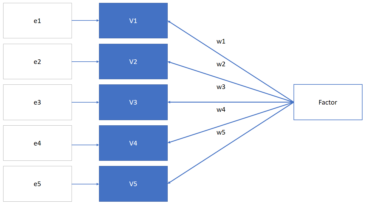
Thus, in factor analysis we may use: \(V_i = w_i*Factor + e_i\)
PCA allows you to reduce the numb er of variables as a liner combination of the minimum number of factors 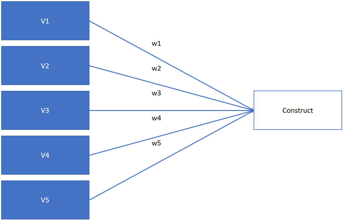
Thus, in PCA we may use: \(Construct=V_1w_1+V_2w_2+V_3w_3+V_4w_4+V_5w_5\)
Note: There are other approaches to compute the value for the construct (e.g., linear regression). We will discuss those later in the tutorial.
Conducting Factor Analysis and PCA
Correlation among items
As we said before, the first thing we need to do is to compute the correlation among items to see if there is an actual underlying structure to the data
The function rcorr from the Hmisc package allow us to compute these correlations from a matrix. In the following box, we first read our dataset (items in columns, and subjects in rows) and then compute the correlation among items.
We will use the sample dataset bfi: “25 personality self report items taken from the International Personality Item Pool (ipip.ori.org) were included as part of the Synthetic Aperture Personality Assessment (SAPA) web based personality assessment project. The data from 2800 subjects are included here as a demonstration set for scale construction, factor analysis, and Item Response Theory analysis. Three additional demographic variables (sex, education, and age) are also included.”
For more information about this dataset: https://www.personality-project.org/r/html/bfi.html
For this example, we will only use 15 items, corresponding to three factors.
surveyData<- bfi[,1:15]
corResults <- rcorr(as.matrix(surveyData))
KMO(corResults$r)
MSA
We now use the KMO function with the correlation results to compute the measure of sampling adequacy (MSA).
Remeber that the interpretation of this statistic is as follow: * MSA > 0.8 Meritorious * MSA > 0.7 Middling * MSA > 0.6 Mediocre * MSA > 0.5 Miserable * MSA < 0.5 Unacceptable.
Practice Activity
Practice Activity
Remove the items with a MSA below 0.8 one by one, and compute the KMO again.
Hint: To remove an item from a dataset, use the minus symbol and the number of the column. For instance, if you want to remove the 10th column, you would use: surveyData[,-10].
Use the appropriate column number to remove the one we do not want to include in the analysis.
# Insert your code hereTwo additional cosiderations to conduct factor analysis and PCA
Number of Factors
Factors are extracted one by one, where the first one represents the best summary of the variance; the second factor is the second best one but must be orthogonal (i.e., extracted from the remaining shared variance) to the first factor.
The eigenvalue of each factor represents the percentage of variance explained by that factor as compared to an individual item. In other words, if the eigen value of a factor is larger than 1, it means that such factor explains more than one individual item.
There are different methods to identify the number of factors for our data:
Latent root criterion: Eigenvalue larger than 1. The factor accounts for at least the variance of one variable.
Percentage of variance: in the social sciences, the total variance explained should be 60% or more.
Scree test: The scree plot compares the eigenvalues (y-values) to the number of factors (X-axis). When there is a small drop in the eigenvalues between i and i+1 factors (i.e., an elbow), we can decide to extract i factors. The plot looks like this:
 Source: https://commons.wikimedia.org/wiki/File:Screeplotr.png
Rotation Method
When conducting factor analysis, we rotate the axes either orthogonally or obliquely to redistribute the remaining variance, achieving a more meaningful factor pattern.
- Some Orthogonal Rotation Methods We use these rotation methods when the factors are correlated to each other
- Quartimax: Simplify the rows variable loads high on one factor and low on all others. Problem: tends to create a general factor with most variables with high loadings.
- Varimax: Simplify the columns, maximizes the sum of variances of required loadings. Maximizes dispersion of loadings within factors.
- Some Oblique Rotation Methods: We use these rotation methods when the factors are correlated to each other
- Oblimin: Standar oblique rotation method.
- Promax: useful for large datasets
Factor Analysis
To conduct exploratory factor analysis, we can use the function fa from the package psych. Note that we can also plot how our items distribute between the dimensions that represent our factors using the function plot.psych
Remember that we wanted to remove a few columns from the dataset. We use the following instruction to exclude the column for A1. Execute the following code and think about these things:
What is the percentage of variance explained by this model?
Are two factors enough to explain our variances?
Hint: Here are some tips to where to look for this information. 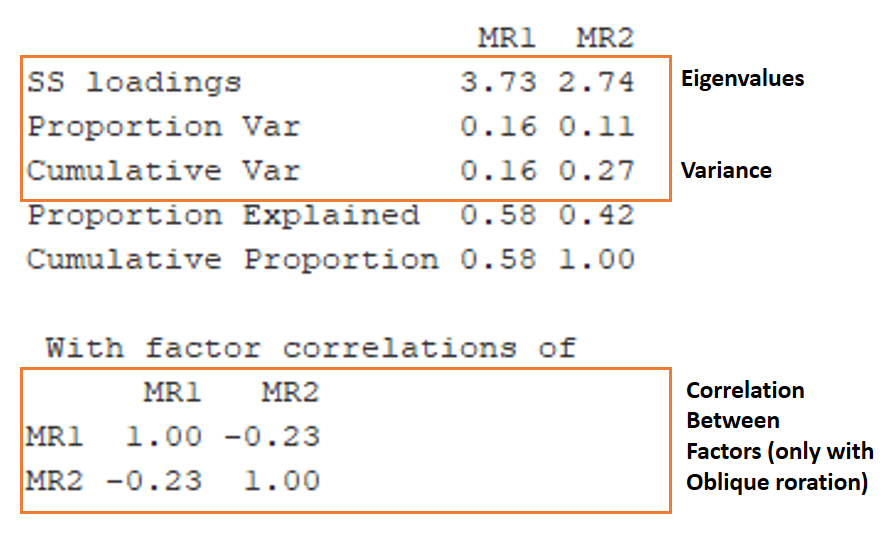
faResults<-fa(surveyData[, -1], nfactors = 2, rotate = 'varimax' )
faResults
plot.psych(faResults)
Practice Activity
In the example, we used 2 factors and the rotation method varimax. In this activity you should:
Try different number of factors, check the eigenvalues, and make an informed decision about the number of factors to extract
Try different rotation methods, and see which one works best. Hint: The correlation among factors is only showed when we use oblique rotation methods.
Use the following function to create a Scree Plot and choose a number of factors
scree(corResults$r)
# Insert your code herePCA
Let’s now conduct PCA with the same dataset. Again, we start with two factors and the varimax rotation.
Note, however, that we use the correlation results (the r matrix), instead of the original dataset.
pc <- principal(corResults$r,2,rotate="varimax")
print.psych(pc, cut=0.4, sort=TRUE)
plot.psych(pc)
Practice Activity
Complete the same activity that you did for factor analysis (changing number of factors and rotation methods.)
Compare the results from factor analysis and principal component analysis.